R, the Programmable Web, and Transparency in Social Science Research

Alois Stutzer and I recently contributed a guest post to the BITSS-Blog (of the Berkeley Initiative for Transparency in the Social Sciences). As a big part of it focuses on R-related topics, I figured it might also be of interest for readers of this blog. Here the gist:

"The replicability of social science research is becoming more demanding in the age of big data. First, researchers aiming to replicate a study based on massive data face substantial computational costs. Second, and probably more challenging, they are often confronted with “highly unique” data sets derived and compiled from sources with different and unusual formats (as they are originally generated and recorded for purposes other than data analysis or research). This holds in particular for Internet data from social media, new e-businesses, and digital government. More and more social scientists attempt to exploit these new data sources following ad hoc procedures in the compilation of their data sets. 
..."

The entire post can be found here.

In this context, I also want to explicitly point to all the very relevant contributions listed in the CRAN Task View on Web Technologies and Services,  the CRAN Open Data Task View, as well as the contributions by rOpenSci.

Easy access to data on US politics: New version of pvsR now on BitBucket

I am happy to announce a new release (version 0.4) of the R-package pvsR  on Bitbucket. pvsR facilitates data retrieval from Project Vote Smart's rich online data base on US politics via the Project Vote Smart application programming interface (PVS API). The functions in this package cover most PVS API classes and methods and return the requested data in data-frames (and classes "tbl_df", "tbl"). See here for extended examples and background. The new version includes the following improvements:

• Replaced internal function dfList() with faster implementation in dplyr::bind_rows, removed dfList() from package.
• In order to improve the comfort in interactive sessions, all high-level functions for querying data from the PVS API return now objects of class "tbl_df"/"tbl"/"data.frame".
• Improved code-readability/formatting.

How to install/use

# install/load package
library(devtools)
install_bitbucket("ulrich-matter/pvsR")
library(pvsR)
 
# define api-key variable (use personal key, see http://votesmart.org/share/api)
pvs.key <- "<YOUR-KEY-HERE>"
 
# get biographical data on Hilary Clinton and Donald Trump
Candidates.getByLastname(list("Clinton", "Trump"))

Created by Pretty R at inside-R.org

Suggestions and issue reports very welcome

 

Please feel free to  make suggestions, and report issues (preferably via the issue-tracker in the Bitbucket-repository).

RWebData V. 0.1 on Bitbucket: A High-Level Interface to the Programmable Web

I am happy to announce the first release of the R-package RWebData  on Bitbucket. The main aim of the package is to provide high-level functions that facilitate the access and systematic collection of data from REST APIs for the purpose of statistical analysis. RWebData is thus made for users that predominantly use R as a statistical software but do not have experience with web APIs and/or web data formats. In a broader sense (and in the long run) the package should serve as a high level interface to the programmable web for research in the social sciences (i.e., accessing the programmable web as a data source). The package thus takes up some of the broader ideas discussed in our paper on the pvsR-package. A short paper with a broader motivation for the package, some discussion of the package's architecture, as well as a practical introduction with several examples can be found here.

RWebData builds on many important packages that facilitate client-server interaction via R/HTTP as well as different parsers for web-data formats (including: RCurl, jsonlite, XML, XML2R, httr, mime, yaml, RJSONIO). At its core, the package provides a generic approach to map nested web data to a flat data representation in the form of one or several (non-nested) data-frames. 

A simple example

This example is taken from the working paper on arXiv. It illustrates the very basic usage of the package: Say you want to statistically analyze/visualize data provided from a web API, all you have is an URL pointing to the data of interest, you do not know/care what JSON, XML and the like are, you simply want the data in a format that is suitable for statistical analysis in R. 

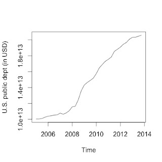
Here, we want to fetch data from the World Bank Indicators API which provides time series data on financial indicators of different countries (as XML in a compressed text file). In the example, we query data from that API in order to investigate how the United States' public dept was affected by the financial crisis in 2008.

# install the package directly from bitbucket
library(devtools)
install_bitbucket('ulrich-matter/RWebData')
library(RWebData)
 
# fetch the data and map it to a table-like representation (a data-frame)
u <- "http://api.worldbank.org/countries/USA/indicators/DP.DOD.DECN.CR.GG.CD?&date=2005Q1:2013Q4"
usdept <- getTabularData(u)
 
# analyze/visualize the data
require(zoo)
plot(as.ts(zoo(usdept$value,  as.yearqtr(usdept$date))), 
     ylab="U.S. public dept (in USD)")

Created by Pretty R at inside-R.org

More examples will follow...

Comments etc. very welcome

Please feel free to comment, make suggestions, and report issues (preferably via the issue-tracker in the Bitbucket-repository). As mentioned above, this is the first release. While I have already used the package to collect data for several of my own research projects, there are certainly still a lot of issues to be resolved...

Data Science in Business/Computational Social Science in Academia?

Nomen Est Omen?

Lately, the terms "data science" and "data scientist" turn up at an increasing pace in the R-blog-sphere. Since its first occurrence (to my knowledge,  "data scientist" has been coined by DJ Patil and Jeff Hammerbacher in 2008), the term "data scientist" has become established and accepted not only in the data-blog-sphere but also in the corporate/business world as well as in academia. It's frequent occurrence as job title as well as some controversial discussions on the situation of the respective labor market are evidence for our understanding of data scientist as an occupational title. At the same time data science is being established as a course taught at universities (with the first drafts of specific textbooks to learn data science; see, e.g., Jeffrey Stanton's free book on data science).   Interestingly, by the existence of job descriptions for data scientists and the respective skill sets, our understanding of data science is increasingly defined through what the corporate labor market demands - hence, through business. As I see it, this development is also taken up by the scholars teaching data science at universities. A data science course is quite specifically a preparation for a future job as data scientist. In that sense, data science is not a science itself but the application of various sciences (computer science, statistics, etc.). This notion, I think, is also present when reading the JDS.

Empirical Computational Social Science

 The corporate labor market asks for data scientists and universities are offering new courses in order to fill the gaps. But, is there also room for data science skills in a purely academic research environment?

I think, there is very much room for it. At around the same time the term "data scientist" came up, the Science Magazine published Lazer et al.'s maniphesto on data-driven computational social science (or, the term I prefer, empirical computational social science). Historically, the term computational social science is rather referring to the application of numerical methods and simulation (i.e., agent based modelling) to complex issues of social science research. What Lazer et al. rather understand as computational social science, however, is social science research that draws on the enormous potential of vast amounts of digital data on social interactions (made available through the Internet, mobile applications etc.). Handling this data in order to conduct empirical social science research clearly needs data science skills. To come full circle, I have revisited Drew Conway's post and Venn-diagram on data science and drafted another Venn-diagram to illustrate how data-driven computational social science could be interpreted in the framework discussed above.

Whether or not you generally share my point of view concerning data science and computational social science, I am pretty sure you will agree on one thing: R will play an important role in the further development of these fields.

My R-Package Development Cheat Sheet

In case you have no experience in writing an R-package yourself  but would like to start developing one right away, this post might be helpful.

I'm about to finish my first own (serious) R-package these days (more on the package itself later). While writing my package, I collected a handful of commands and notes etc. that proofed to be helpful, and saved them in a R-script. I usually had that script open in one window when writing/testing some parts of my package in RStudio. I figured that it might help someone in a similar situation. Note, though, that this little code collection has no ambitions whatsoever to be anything like a complete guide to develop your own R-package. Having that said, here it is (you can also download it from my github repo):

#######################################################
# This was contributed by giventhedata.blogspot.com   #
#######################################################
 
 
# I. Very useful tools when writing a R-package:
#------------------------------------------------
install.packages("devtools", "roxygen2")
library(devtools)
library(roxygen2)
 
 
# II. getting started
#--------------------
 
# assuming your package is to be called 'MyRpackage' and
# all the scripts that contain functions that should be part
# of your package are in your current working directory and
# and there are no functions loaded in the workspace of your 
# current R-session...
 
# source all scripts:
myscripts <- c("script1.R", "script2.R", "script3.R") #...
 
for (i in myscripts) source(i)
 
 
# get all the names of the functions in the workspace
fs <- c(lsf.str()) 
 
# create package skeleton:
package.skeleton("MyRpackage", fs)
 
 
# III. While working on your package...
#--------------------------------------
 
# renew documentation
MyRpackage_package <- as.package("MyRpackage")
document(MyRpackage_package)
 
# build and check
system("R CMD build MyRpackage")
system("R CMD check MyRpackage")
system("R CMD Rd2pdf MyRpackage") # update/check manual.pdf (while working on the documentation)
 
# install your package from the local directory after successfully building it
install.packages(paste(getwd(),"/MyRpackage_0.1.tar.gz",sep=""), repos=NULL, type="source")
 
# load it for tests
library(MyRpackage)
 
# unload old version of package after changes (in order to install new built)
detach(package:MyRpackage, unload=TRUE)
 
 
#Note:
# For internal functions: delete Rd-file, leave out export-command in Namespace

Syntax highlighting created by Pretty R at inside-R.org

Estimating Pi with R via MCS-Dart: A very simple example of numerical integration, illustrated and computed in R.

Have you ever played Monte Carlo Dart? If not, read this post and learn how to do it with R and what it can be used for. In fact it is a very easy and prevalent example (which I have come across in a  computational economics course last spring semester) that demonstrates the idea behind numerical integration. The aim of this post is not to present a programmatically swell implementation but rather to give an illustrative explanation. Having that said, here's the problem:

You know of the existence of the number Pi and its role in determining the area of a circle. But, you don't know its value. How can you estimate the value of Pi using Monte Carlo Simulation, or in other words using random numbers?

Square and circle

First, draw a circle with radius r=1 placed in a square with side length a=2r=2 to illustrate the initial setting. Note that I use the shape package to draw the circle.

library(shape)

r <- 1

par(pty="s")

emptyplot(c(0, 0),frame.plot=r)

plotcircle(r=r, mid=c(0,0), lwd=1,lcol="blue")

lines(x=c(0,1),y=c(0,0), lty=1, col="red")

lines(x=c(-1,1),y=c(0,0), lty=2)

lines(y=c(-1,1),x=c(0,0), lty=2)

axis(1)

axis(2)

text(x=0.5,y=0.2, labels=expression("r=1"), col="red")

Generally, if a circle with radius r is surrounded by a square with side length a=2r, Pi is equal to the area of the circle divided by the area of the square times 4. Hence, by estimating the fraction of the two areas multiplied by 4 we estimate the value of Pi.

# in case you want to plot the math in R...

emptyplot( xlim=c(0,10), ylim=c(0,11))

text(5,10, expression(paste(A[circle] == r^2 %*% pi, "  and  ", A[square] == (2 * r)^{2},"; ", sep="") ))

text(5,7, expression( paste( frac(A[circle], A[square]) == frac(r^2 %*% pi, (2 * r)^{2}), " = ", frac(pi, 4), ";  thus  ", 4 %*% frac(A[circle], A[square]) == pi, sep="") ))

Playing Monte Carlo Dart

To estimate the fraction of the two areas, we use Monte Carlo Simulation. Imagine it (in this context) as a simulation of randomly throwing darts at the graph above and check for each dart whether it is inside or outside of the circle. The fraction of darts inside the circle is approximately the area of the circle relative to the area of the square (and thus, multiplied by 4, approximately the value of Pi). Intuitively this approximation gets better the greater the number of darts (random numbers) is. But even with a high number of darts the estimated value might in one execution of the experiment be above and in another under the true value of Pi. On average the estimated value is, though, unbiased and pretty close to the real value. Hence, to get a fair estimation we repeat the experiment many times and take the mean of the results.

In fact, the approach described above can be even more simplified. Instead of looking at the whole circle/square it is sufficient to only look in the upper right fourth of the circle/square (as illustrated below). With that target we do exactly the same "dart-throwing" and multiply the resulting fraction by 4.

r <- 1

par(pty="s")

emptyplot(frame.plot=r)

plotcircle(r=r, mid=c(0,0), lwd=1,lcol="blue")

lines(x=c(0,1),y=c(0,0), lty=1, col="red")

lines(x=c(-1,1),y=c(0,0), lty=2)

lines(y=c(-1,1),x=c(0,0), lty=2)

axis(1)

axis(2)

How to "throw the darts"?

We draw two vectors of random numbers that are ~U(0,1). One for the x coordinates and one for the y coordinates. Each combination of the elements of these two vectors gives us the location where a "dart hit the target". The remaining question is how to determine whether the dart hit the square inside or outside the circle. The answer comes from the Pythagorean theorem. Imagine the distances from the axes to the point (0.8,0.58) as side lengths a and b of a triangle. If the value of the unknown side length c is greater than the radius r (1), the point is outside the circle; otherwise it is inside (or on) the circle (see illustration below).

 

# Illustration Pythagorean

par(pty="s")

emptyplot(frame.plot=r)

plotcircle(r=r, mid=c(0,0), lwd=1,lcol="blue")

lines(x=c(0,1),y=c(0,0), lty=1, col="red")

lines(x=c(-1,1),y=c(0,0), lty=2)

lines(y=c(-1,1),x=c(0,0), lty=2)

axis(1)

axis(2)

points(x=0.8,y=0.58,col="red", lwd=2)

lines(x=c(0,0.8), y=c(0,0), col="red", lwd=2)

lines(x=c(0.8,0.8), y=c(0,0.58), col="red", lwd=2)

lines(x=c(0,0.8), y=c(0,0.58), col="red", lty=2,lwd=2)

text(x=0.4,y=0.4,"c",col="red")

title(expression(c == sqrt(a^2 + b^2)))

A function for one round of Monte Carlo Dart

The following function estimates Pi with the approach described above. The only input to the function is the number of "darts" (random coordinates) n. Note that this implementation is programmatically not smart because it uses a loop instead of vectorization. But, I think it is more illustrative for (R-) programming beginners this way.
  

est.pi <- function(n){
inside <- 0
outside <-0

pi.est <- 0

# draw random numbers for the coordinates of the "dart-hits"

a <- runif(n,0,1)
b <- runif(n,0,1)

# use the pythagorean theorem

c <- sqrt((a^2) + (b^2) )

# loop: check for each point whether it is inside or outside the circle:

for (i in 1:n) {
   
   if (c[i] > 1) {

     

      outside <- outside + 1

     

    } else {

     

      inside <- inside + 1

     

    }

       

    if (i==n) {pi.est <- (inside/(inside+outside))*4} # compute an estimation of the value of pi

    

  }

 return(pi.est)

}

Try that function several times. For the same n you will every time get different estimations of the value of Pi. That is due to the fact, that the whole approach is based on random numbers.

   

est.pi(n=1000)

est.pi(n=1000)

est.pi(n=1000)

Now, repeat this experiment 1000 times and take the mean of the results as an unbiased estimation of the value of pi. Compare the result with the value of Pi defined in R.

   

rep <- 1000

pis <- sapply(1:rep, function(x){

  est.pi(n=1000)

})

mean(pis)

pi # value of pi defined in R

Finally, get a graphical overview of the estimation.

  

plot(density(pis), main=expression(paste("Distribution of estimated ",pi,"-values")),cex.main=0.7, cex.axis=0.7, cex.lab=0.7)

# the value of pi defined in R

lines(x=c(pi,pi),y=c(0,10), lty=1,col="blue")
# the estimation

lines(x=c(mean(pis),mean(pis)),y=c(0,10), lty=1,col="red")

What has this to do with numerical integration?

The link between the application of "MCS-Dart" to estimate the value of Pi and the general idea behind numerical integration is straightforward. The core of the approach described above is to draw random numbers (of a certain interval) for coordinates and check, whether the resulting points are under or above a curve. If one is interested in the (approximate) area under a curve of a given function y=f(x) =... in a certain interval and it is very hard to find the integral analytically one can apply exactly the same approach. Draw random numbers for x and y, check if y is greater than f(x), if so, the point (x,y) must be above the curve and otherwise under the curve. Compute the fraction of points under the curve and multiply it by the total area of the rectangle with the x- and y-intervals as side lengths...

R and the web (for beginners), Part III: Scraping MPs' expenses in detail from the web

In this last post of my little series (see my latest post) on R and the web I explain how to extract data of a website (web scraping/screen scraping) with R. If the data you want to analyze are a part of a web page, for example a HTML-table (or hundreds of them) it might be very time-consuming (and boring!) to manually copy/paste all of its content or even typewrite it to a spreadsheet table or data frame. Instead, you can let R do the job for you!

This post is really aimed at beginners. Thus, to keep things simple it only deals with scraping one data table from one web page: a table published by BBC NEWS containing the full range of British Members of Parliament' expenses in 2007-2008. Quite an interesting data set if you are into political scandals...

Web scraping with R

There are several R packages that might be helpful for web scraping, such as XML, RCurl, and scrapeR. In this example only the XML package is used. As a fist step, you parse the whole HTML-file and extract all HTML-tables in it:

library(XML)

# URL of interest:
mps <- "http://news.bbc.co.uk/2/hi/uk_politics/8044207.stm" 

# parse the document for R representation:
mps.doc <- htmlParse(mps)

# get all the tables in mps.doc as data frames

mps.tabs <- readHTMLTable(mps.doc) 

mps.tabs is a list containing in each element a HTML-table from the parsed website (mps.doc) as data.frame. The website contains several HTML-tables (some are rather used to structure the website and not to present data). The list mps.tabs actually has seven entries, hence there were seven HTML-tables in the parsed document:

length(mps.tabs)

To proceed you need to check which of these data frames (list entries) contains the table you want (the MPs' expenses). You can do that "manually" by checking how the data frame starts and ends and compare it with the original table of the website:

head(mps.tabs[[1]])  #and

tail(mps.tabs[[1]])  #for 1 to 7

With only seven entries this is quite fast. But alternatively you could also write a little loop to do the job for you. The loop checks each data frame for certain conditions. In this case: the string of the first row and first column and the string in the last row and column. According to the original table from the website that should be:

first <- "Abbott, Ms Diane"

last <- "157,841"

# ... and the loop:

for (i in 1:length(mps.tabs)) {

 

  lastrow <- nrow(mps.tabs[[i]]) # get number of rows

  lastcol <- ncol(mps.tabs[[i]])

 

  if (as.character(mps.tabs[[i]][1,1])==first & as.character(mps.tabs[[i]][lastrow,lastcol])==last) {

   

    tabi <- i

     

    }

  }

Check if that is realy what you want and extract the relevant table as data frame.

head(mps.tabs[[tabi]])

tail(mps.tabs[[tabi]])

mps <- mps.tabs[[tabi]] 

Before you can properly analyze this data set we have to remove the commas in the columns with expenses and format them as numeric:

money <- sapply(mps[,-1:-3], FUN= function(x) as.numeric(gsub(",", "", as.character(x), fixed = TRUE) ))

mps2 <- cbind(mps[,1:3],money)

Now you are ready to go... For example, you could compare how the total expenses are distributed for each of the five biggest parties:

# which are the five biggest parties by # of mps?

nbig5 <- names(summary(mps2$Party)[order(summary(mps2$Party)*-1)][1:5])

#subset of mps only with the five biggest parties:

big5 <- subset(mps2, mps$Party%in%nbig5)

# load the lattice package for a nice plot

library(lattice)

bwplot(Total ~  Party, data=big5, ylab="Total expenses per MP (in £)")

Here is the resulting plot: 

 And the relevant R code in one piece:

library(XML)

# URL of interest:
mps <- "http://news.bbc.co.uk/2/hi/uk_politics/8044207.stm" 

# parse the document for R representation:
mps.doc <- htmlParse(mps)

# get all the tables in mps.doc as data frames

mps.tabs <- readHTMLTable(mps.doc)

# loop to find relevant table:

first <- "Abbott, Ms Diane"

last <- "157,841"

for (i in 1:length(mps.tabs)) {

 

  lastrow <- nrow(mps.tabs[[i]]) # get number of rows

  lastcol <- ncol(mps.tabs[[i]])

 

  if (as.character(mps.tabs[[i]][1,1])==first & as.character(mps.tabs[[i]][lastrow,lastcol])==last) {

   

    tabi <- i

     

    }

  }


# extract the relevant table and format it:

mps <- mps.tabs[[tabi]]  

money <- sapply(mps[,-1:-3], FUN= function(x) as.numeric(gsub(",", "", as.character(x), fixed = TRUE) ))

mps2 <- cbind(mps[,1:3],money)

# which are the five biggest parties by # of mps?

nbig5 <- names(summary(mps2$Party)[order(summary(mps2$Party)*-1)][1:5])

#subset of mps only with the five biggest parties:

big5 <- subset(mps2, mps$Party%in%nbig5)

# load the lattice package for a nice plot

library(lattice)

bwplot(Total ~  Party, data=big5, ylab="Total expenses per MP (in £)")

 More web scraping examples on r-bloggers.com

If you are interested in more web scraping with R, check out the following links to posts with more advanced/specific examples presented on r-bloggers.com:

http://www.r-bloggers.com/web-scraper-for-google-scholar-updated/ 

http://www.r-bloggers.com/web-scraping-in-r/

http://www.r-bloggers.com/r-web-scraping-r-bloggers-facebook-page-to-gain-further-information-about-an-authors%E2%80%99-r-blog-posts-e-g-number-of-likes-comments-shares-etc/

http://www.r-bloggers.com/web-scraping-yahoo-search-page-via-xpath/

http://www.r-bloggers.com/how-to-buy-a-used-car-with-r-part-1/